What is NeRF?

NeRF (Mildenhall, Srinivasan, Tancik et al. (2020)) or Neural Radiance Field is a deep learning approach to volume rendering. A NeRF is able to synthesize novel views of 3D scenes given a sparse set of input views.

Volume rendering

To better understand NeRF, we must first grasp the concept of volume rendering and the relevant mathematical equations. This section is based on what should have been the appendix to NeRF: Volume Rendering Digest (for NeRF).

Volume rendering is a technique for visualizing 3D data by projecting it into a 2D image plane.

Rendering Equations

In NeRF the rendering equations assume that the scene is composed of a volume with absorption and emission but no scattering. (see Scratchapixel: Volume Rendering for Developers: Foundations and The Physically Based Rendering Book Section 11.1 for more details on volume rendering)

The color of a pixel in an image is the expected value of the light emitted by particles in the volume as the ray corresponding to that pixel travels through the volume:

$$C(\mathbf{r})= \mathbb{E}_{\text{ray }\mathbf{r} \text{ hitting particle at distance } t} [\mathbf{c}(\mathbf{r}(t))]$$

Given volume density $\sigma(\mathbf{x})$ with $\mathbf{x} \in \mathbb{R}^3$, which is defined as the differential likelihood of a ray hitting a particle (while traveling an infinitesimal distance) and the transmittance function $\mathcal{T}(t)$, which indicates the probability of a ray traveling over the interval $[0, t)$ without hitting any particles. Then $\mathcal{T}(t) \cdot \sigma(t)$ can be interpreted as the probability density function that gives the likely hood that the ray stops precisely at distance $t$.

We can now rewrite the exepected color as: $$C(\mathbf{r})= \int_0^D \mathcal{T}\cdot\sigma(\mathbf{r}(t))\cdot\mathbf{c}(\mathbf{r}(t)) dt$$ with $D$ the distance that the ray travels. Without loss of generality, we omitted the influence of a background color.

Transmittance funtion: The transmittance function can be defined in terms of the density. If $\mathcal{T}(t)$ indicates the probability of a ray traveling over the interval $[0,t)$ then $\mathcal{t}(t + dt)$ is equal to $\mathcal{T}(t)$ times the probabiliy of not hitting a particle over step $dt$ which is $(1 - dt \cdot \sigma(\mathbf{r}(t))$. $$ \begin{aligned} \mathcal{T}(t+dt) =& \mathcal{T}(t) \cdot (1 - dt \cdot \sigma(\mathbf{r}(t))) & \\ \frac{\mathcal{T}(t+dt) - \mathcal{T}(t)}{dt} \equiv& \mathcal{T}’(t) = -\mathcal{T}(t) \cdot \sigma(\mathbf{r}(t)) & \\ \mathcal{T}’(t) &= -\mathcal{T}(t) \cdot \sigma(\mathbf{r}(t)) & \scriptstyle{\text{; solve as differential equation}} \\ \frac{\mathcal{T}’(t)}{\mathcal{T}(t)} &= -\sigma(\mathbf{r}(t)) & \\ \int_a^b \frac{\mathcal{T}’(t)}{\mathcal{T}(t)} \; dt &= -\int_a^b \sigma(\mathbf{r}(t)) \; dt & \scriptstyle{\text{; take integral from a to b}} \\ \log \mathcal{T}(b) - \log \mathcal{T}(a) &= -\int_a^b \sigma(\mathbf{r}(t)) \; dt & \scriptstyle{\text{; solve left side}} \\ \log \left(\frac{\mathcal{T}(b)}{\mathcal{T}(a)}\right) &= -\int_a^b \sigma(\mathbf{r}(t)) \; dt & \\ \mathcal{T}(a \rightarrow b) \equiv \frac{\mathcal{T}(b)}{\mathcal{T}(a)} &= \exp\left({-\int_a^b \sigma(\mathbf{r}(t)) \; dt}\right) & \end{aligned} $$

Combining this gives us the formula $(1)$ from the paper. $$C(\mathbf{r}) = \int_{t_n}^{t_f}T(t)\sigma(\mathbf{r}(t))\mathbf{c}(\mathbf{r}(t),\mathbf{d})\;dt\,, \textrm{ where }T(t) = \exp({-\int_{t_n}^{t}\sigma(\mathbf{r}(s))\;ds})$$ with the difference that the color $\mathbf{c}$ of a particle not only depends on the location but also on the viewing direction.

In order to get rid of the integrals, we assume piecewise constant density and color. This simplifies the equation to: $$ \begin{aligned} C(\mathbf{r})\approx& \sum_{i=1}^N \sigma_i \cdot \mathbf{c}_i \cdot \int_{t_i}^{t_{i+1}} \mathcal{T}(t) \; dt &\scriptstyle{\text{; piecewise constant density and color}} \\ \hat{C}(\mathbf{r}) =& \sum_{i=1}^N \sigma_i \cdot \mathbf{c}_i \cdot \int_{t_i}^{t_{i+1}} \exp \left( - \int_{t_n}^{t_i} \sigma_i \, ds \right) \exp \left( - \int_{t_i}^{t} \sigma_i \, ds \right) \, dt & \scriptstyle{\text{; split transmittance}} \\ =& \sum_{i=1}^N \sigma_i \cdot \mathbf{c}_i \cdot \int_{t_i}^{t_{i+1}} \exp \left( - \sum_{j=1}^{i-1} \sigma_j \delta_j \right) \exp \left( - \sigma_i ( t - t_i) \right) \, dt & \scriptstyle{\text{; piecewise constant density}} \\ =& \sum_{i=1}^N \mathcal{T}_i \cdot \sigma_i \cdot \mathbf{c}_i \cdot \int_{t_i}^{t_{i+1}} \exp( - \sigma_i ( t - t_i)) \, dt & \scriptstyle{\text{; }\mathcal{T}_i = \exp \left( - \sum_{j=1}^{i-1} \sigma_j \delta_j \right)\text{ and constant}} \\ =& \sum_{i=1}^N \mathcal{T}_i \cdot \sigma_i \cdot \mathbf{c}_i \cdot \frac{\exp( - \sigma_i (t_{i+1} - t_i)) - 1}{-\sigma_i} & \scriptstyle{\text{; solve integral}} \\ =& \sum_{i=1}^N \mathcal{T}_i \cdot \mathbf{c}_i \cdot (1 -\exp( - \sigma_i \delta_i)) & \scriptstyle{\text{; cancel }\sigma_i} \\ \end{aligned} $$

This is equal to formula $(3)$ in the paper.

NeRF overview

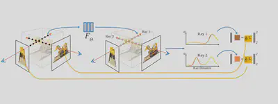
NeRFs represent a scene using a neural network. The input of this neural network is the location of a point $\mathbf{x} \in \mathbb{R}^3$ along a viewing ray (can be expressed as 2D viewing directions)¹. The output of the neural network is the color $\mathbf{c}(\mathbf{x})$ and density $\sigma(\mathbf{x})$ of that point along the ray. By sampling multiple points along a certain ray, and using the rendering functions as defined earlier the predicted color a pixel in an input image can be reconstructed. As this entire process is differentiable, NeRFs learn the color and density fields of a scene.

The details

From images to neural network inputs

Neural radiance fields do not take images as direct inputs. Instead, they work with camera rays that correspond to each pixel in an image. These rays can be computed from the camera’s intrinsic and extrinsic matrices, which describe its position, orientation, and focal length.

Once the camera rays are computed, they can be used to sample points along the ray. However using the 3D coordinates of these points as input does not work well. Instead, the authors proposed to use positional encodings to map the inputs to a higher dimensional space. More specifically, the authors used the following positional encoding: $$\operatorname{PE}(\mathbf{x}) = (\sin(2^0 \pi \mathbf{x}), \cos(2^0 \pi \mathbf{x}), \ldots, \sin(2^{N-1} \pi \mathbf{x}), \cos(2^{N-1} \pi \mathbf{x}))$$ where $N$ is the dimensionality of the final vector $\mathbf{x’}$.

The authors of NeRF used a hierarchical sampling strategy to sample points along the ray. Ray points are sampled in two stages. First, a set of coarse points are sampled along the ray. These points are sampled uniformly in the interval $[t_{near}, t_{far}]$ where $t_{near}$ and $t_{far}$ are the distances to the nearest and farthest points along the ray that are visible to the camera. However, most points sampled this way will be empty space. To reduce the number of empty space points, the authors used a second stage of sampling. Given the output of the neural network at the coarse points, the network is used to predict the density $\sigma$ of the points. The fine points are sampled from the piece-wise constant PDF constructed by $\hat{w}_i = \frac{w_i}{\sum_j w_j}$ where $w_i = T_i(1 - \exp(-\sigma_i \delta_i))$ .