Outrageously Large Neural Networks: The Sparsely-Gated Mixture-of-Experts Layer
Draw an overview of the Sparsely Gated Mixture of Experts (MoE) layer.
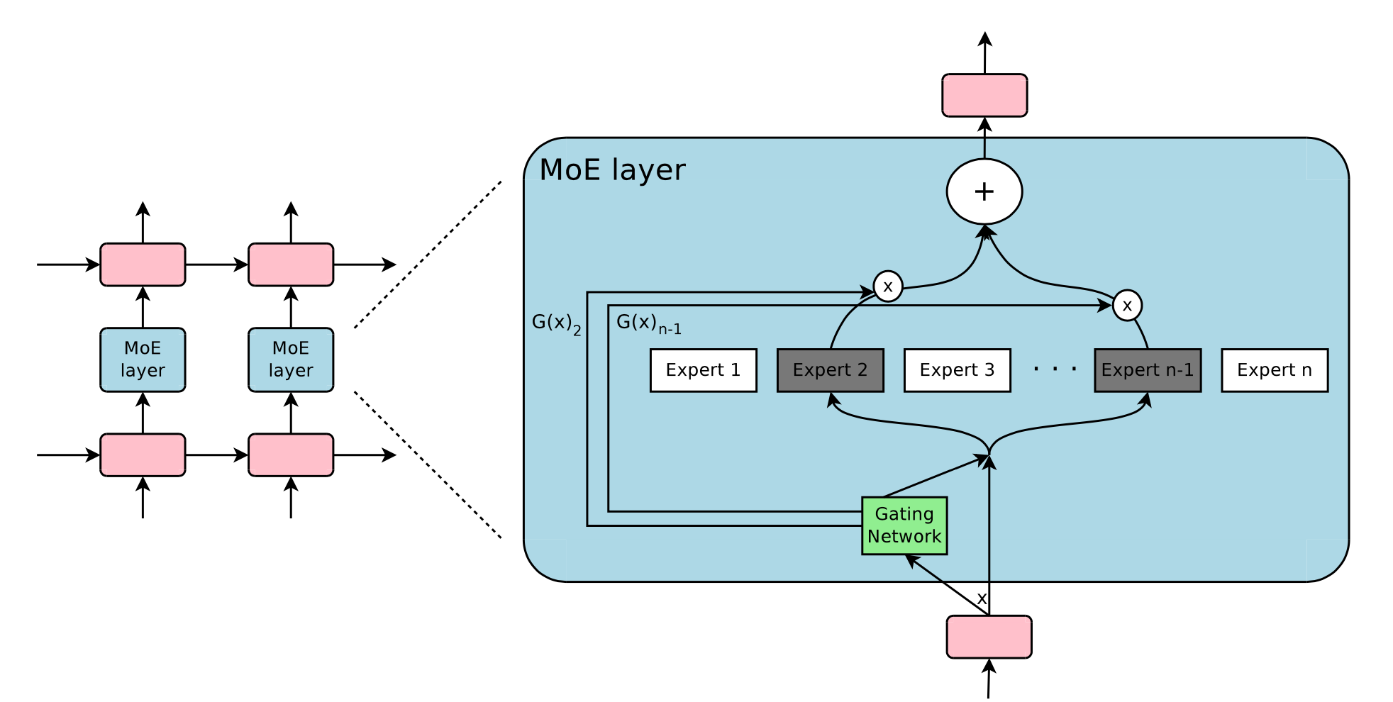
The Mixture-of-Experts layer consists of \(n\) experts (simple feed forward layers in the original paper) and a gating network \(G\) whose output is a sparse \(n\) dimensional vector.
Let us denote by \(G(x)\) and \(E_i(x)\) the output of the gating network and the output of the \(i\)-th expert network for a given input \(x\). The output \(y\) of the MoE module can be written as follows:
\[y = \sum_{i=1}^n G(x)_iE_i(x)\]We save computation based on the sparsity of the output of \(G(x)\).
Give the structure of the gating network \(G\) that is used in Sparsely Gated MoE.
A simple choice of \(G\) is to multiply the input with a trainable weight matrix \(W_g\) and then apply a \(\operatorname{softmax}\): \(G_\sigma (x) = \operatorname{softmax}(x W_g)\).
However we want a sparsely gated MoE where we only evaluate the top-\(k\) experts.
The sparsity serves to save computations.
Thus the MoE layer only keeps the top-\(k\) values:
\[\begin{aligned} G(x) &= \operatorname{softmax}(\operatorname{KeepTopK}(H(x),k)) \\ \operatorname{KeepTopK}(v,k)_i &=\begin{cases} v_i & \text{if }v_i\text{ is in the top }k\text{ elements of }v \\ -\infty & \text{otherwise} \end{cases} \end{aligned}\]and where \(H(x)\) is a linear layer with added tunable Guassian noise such that each expert sees enough training data and we avoid favouring only a few experts for all inputs.
\[H(x)_i = (xW_g)_i + \epsilon \cdot \operatorname{softplus}((xW_\text{noise})_i ); \quad \epsilon \sim \mathcal{N}(0, \mathbf{1})\]
What is the shrinking batch problem in MoEs?
If a MoE uses only \(k\) out of \(n\) experts, then for a batch of size \(b\), each export only receive approximately \(\frac{kb}{n} \ll b\) samples.
Through data and model parallelism this problem can be negated.
How does the Sparsely-Gated MoE paper avoid the gating network \(G\) to always favor the same few strong experts?
They soft constrain the learning with an additional importance loss \(\mathcal{L}_{\text{importance}}\) that encourages all experts to have equal importance.
Where importance is defined as: \(\operatorname{Importance}(X) = \sum_{x \in X} G(x)\)
The importance loss is then defined as the coefficient of variation of the batchwise average importance per expert:
\[\mathcal{L}_{\text{importance}} = \lambda \cdot \operatorname{CV}(\operatorname{Importance}(X))^2\]Where the coefficient of variation CV is defined as the ratio of the standard deviation \(\sigma\) to the mean \(\mu\), \(\operatorname{CV} = \frac{\sigma}{\mu}\).
In the Sparsely gated MoE paper what is the load loss \(\mathcal{L}_{\text{load}}\) and what does it encourage?
The load loss \(\mathcal{L}_{load}\) encourages equal load per expert. It uses a smooth estimator \(Load(X)\) of examples per expert and minimizes:
\[\mathcal{L}_{load}(X) = \lambda_{load} \cdot \operatorname{CV}(Load(X))^2\]
For the full calculation of the load value, check the original paper.