What is the formula for variational lower bound, or evidence lower bound (ELBO) in variational Bayesian methods?
The evidence lower bound (ELBO) is defined as
\[\log p_\theta(\mathbf{x}) - D_\text{KL}( q_\phi(\mathbf{z}\vert\mathbf{x}) \| p_\theta(\mathbf{z}\vert\mathbf{x}) ) = \mathbb{E}_{\mathbf{z}\sim q_\phi(\mathbf{z}\vert\mathbf{x})}\log p_\theta(\mathbf{x}\vert\mathbf{z}) - D_\text{KL}(q_\phi(\mathbf{z}\vert\mathbf{x}) \| p_\theta(\mathbf{z}))\]
The lower bound part in the name comes from the fact that the KL divergence is always non-negative and thus ELBO is the lower bound of \(\log p_\theta (\mathbf{x})\).
Derive the ELBO loss function used for variational inference.
The goal in variational inference is to minimize \(D_\text{KL}( q_\phi(\mathbf{z}\vert\mathbf{x}) | p_\theta(\mathbf{z}\vert\mathbf{x}) )\) with respect to \(\phi\):
\[\begin{aligned} & D_\text{KL}( q_\phi(\mathbf{z}\vert\mathbf{x}) \| p_\theta(\mathbf{z}\vert\mathbf{x}) ) & \\ &=\int q_\phi(\mathbf{z} \vert \mathbf{x}) \log\frac{q_\phi(\mathbf{z} \vert \mathbf{x})}{p_\theta(\mathbf{z} \vert \mathbf{x})} d\mathbf{z} & \\ &=\int q_\phi(\mathbf{z} \vert \mathbf{x}) \log\frac{q_\phi(\mathbf{z} \vert \mathbf{x})p_\theta(\mathbf{x})}{p_\theta(\mathbf{z}, \mathbf{x})} d\mathbf{z} & \scriptstyle{\text{; Because }p(z \vert x) = p(z, x) / p(x)} \\ &=\int q_\phi(\mathbf{z} \vert \mathbf{x}) \big( \log p_\theta(\mathbf{x}) + \log\frac{q_\phi(\mathbf{z} \vert \mathbf{x})}{p_\theta(\mathbf{z}, \mathbf{x})} \big) d\mathbf{z} & \\ &=\log p_\theta(\mathbf{x}) + \int q_\phi(\mathbf{z} \vert \mathbf{x})\log\frac{q_\phi(\mathbf{z} \vert \mathbf{x})}{p_\theta(\mathbf{z}, \mathbf{x})} d\mathbf{z} & \scriptstyle{\text{; Because }\int q(z \vert x) dz = 1}\\ &=\log p_\theta(\mathbf{x}) + \int q_\phi(\mathbf{z} \vert \mathbf{x})\log\frac{q_\phi(\mathbf{z} \vert \mathbf{x})}{p_\theta(\mathbf{x}\vert\mathbf{z})p_\theta(\mathbf{z})} d\mathbf{z} & \scriptstyle{\text{; Because }p(z, x) = p(x \vert z) p(z)} \\ &=\log p_\theta(\mathbf{x}) + \mathbb{E}_{\mathbf{z}\sim q_\phi(\mathbf{z} \vert \mathbf{x})}[\log \frac{q_\phi(\mathbf{z} \vert \mathbf{x})}{p_\theta(\mathbf{z})} - \log p_\theta(\mathbf{x} \vert \mathbf{z})] &\\ &=\log p_\theta(\mathbf{x}) + D_\text{KL}(q_\phi(\mathbf{z}\vert\mathbf{x}) \| p_\theta(\mathbf{z})) - \mathbb{E}_{\mathbf{z}\sim q_\phi(\mathbf{z}\vert\mathbf{x})}\log p_\theta(\mathbf{x}\vert\mathbf{z}) & \end{aligned}\]So we have:
\[D_\text{KL}( q_\phi(\mathbf{z}\vert\mathbf{x}) \| p_\theta(\mathbf{z}\vert\mathbf{x}) ) =\log p_\theta(\mathbf{x}) + D_\text{KL}(q_\phi(\mathbf{z}\vert\mathbf{x}) \| p_\theta(\mathbf{z})) - \mathbb{E}_{\mathbf{z}\sim q_\phi(\mathbf{z}\vert\mathbf{x})}\log p_\theta(\mathbf{x}\vert\mathbf{z})\]
Once rearrange the left and right hand side of the equation,
\[\log p_\theta(\mathbf{x}) - D_\text{KL}( q_\phi(\mathbf{z}\vert\mathbf{x}) \| p_\theta(\mathbf{z}\vert\mathbf{x}) ) = \mathbb{E}_{\mathbf{z}\sim q_\phi(\mathbf{z}\vert\mathbf{x})}\log p_\theta(\mathbf{x}\vert\mathbf{z}) - D_\text{KL}(q_\phi(\mathbf{z}\vert\mathbf{x}) \| p_\theta(\mathbf{z}))\]
The left side of the equation is exactly what we want to maximize when learning the true distributions: we want to maximize the (log-)likelihood of generating real data (that is \(\log p_\theta(\mathbf{x})\)) and also minimize the difference between the real and estimated posterior distributions (the term \(D_\text{KL}\) works like a regularizer). Note that \(p_\theta(\mathbf{x})\) is fixed with respect to \(q_\phi\).
The negation of the above defines our loss function:
\[\begin{aligned}
L_\text{VAE}(\theta, \phi)
&= -\log p_\theta(\mathbf{x}) + D_\text{KL}( q_\phi(\mathbf{z}\vert\mathbf{x}) \| p_\theta(\mathbf{z}\vert\mathbf{x}) )\\
&= - \mathbb{E}_{\mathbf{z} \sim q_\phi(\mathbf{z}\vert\mathbf{x})} \log p_\theta(\mathbf{x}\vert\mathbf{z}) + D_\text{KL}( q_\phi(\mathbf{z}\vert\mathbf{x}) \| p_\theta(\mathbf{z}) ) \\
\theta^{*}, \phi^{*} &= \arg\min_{\theta, \phi} L_\text{VAE}
\end{aligned}\]
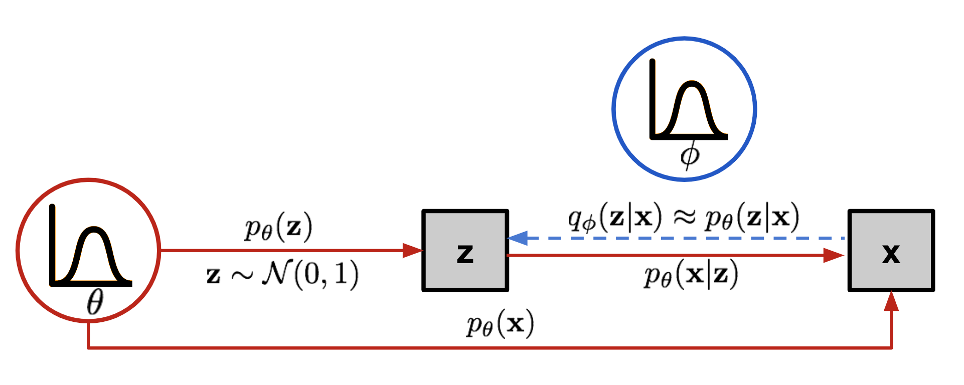
The graphical model involved in Variational Autoencoder. Solid lines denote the generative distribution \(p_\theta(.)\) and dashed lines denote the distribution \(q_\phi(z \mid x)\) to approximate the intractable posterior \(p_\theta(z \mid x)\).
Source: https://lilianweng.github.io/posts/2018-08-12-vae/
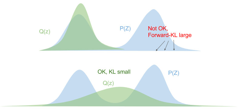
Why does ELBO use the reverse Kullback-Leibler divergence \(D_\text{KL}(q_\phi | p_\theta)\) instead of the forward KL divergence \(D_\text{KL}(p_\theta | q_\phi)\)?
KL divergence is not a symmetric distance function, i.e. \(D_\text{KL}(q_\phi | p_\theta) \ne D_\text{KL}(p_\theta | q_\phi)\).
Let's consider the forward KL divergence:
\[\begin{align*} D_\text{KL}(p | q) & = \sum_z p(z) \log \frac{p(z)}{q(z)} \\ & = \mathbb{E}_{p(z)}{\big[\log \frac{p(z)}{q(z)}\big]}\\ \end{align*}\]This means that we need to ensure that \(q(z) > 0\) wherever \(p(z) > 0\). The optimized variational distribution \(Q(Z)\) is known as zero-avoiding.
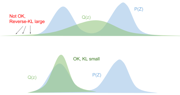
The reversed KL divergence has the opposite behaviour.
\[\begin{align*} D_\text{KL}(q | p) & = \sum_z q(z) \log \frac{q(z)}{p(z)} \\ & = \mathbb{E}_{q(z)}{\big[\log \frac{q(z)}{p(z)}\big]}\\ \end{align*}\]
If \(p(z) = 0\), we must ensure that \(q(z) = 0\), othewise the KL divergence blows up. This is known as zero-forcing.
Let's consider the forward KL divergence:
\[\begin{align*} D_\text{KL}(p | q) & = \sum_z p(z) \log \frac{p(z)}{q(z)} \\ & = \mathbb{E}_{p(z)}{\big[\log \frac{p(z)}{q(z)}\big]}\\ \end{align*}\]This means that we need to ensure that \(q(z) > 0\) wherever \(p(z) > 0\). The optimized variational distribution \(Q(Z)\) is known as zero-avoiding.
The reversed KL divergence has the opposite behaviour.
\[\begin{align*} D_\text{KL}(q | p) & = \sum_z q(z) \log \frac{q(z)}{p(z)} \\ & = \mathbb{E}_{q(z)}{\big[\log \frac{q(z)}{p(z)}\big]}\\ \end{align*}\]
If \(p(z) = 0\), we must ensure that \(q(z) = 0\), othewise the KL divergence blows up. This is known as zero-forcing.
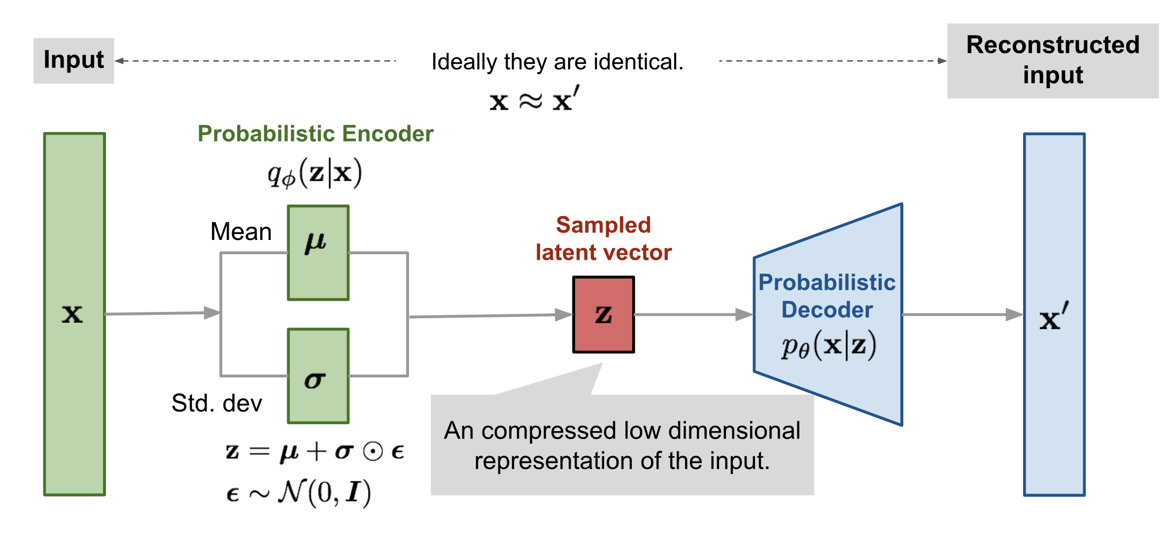
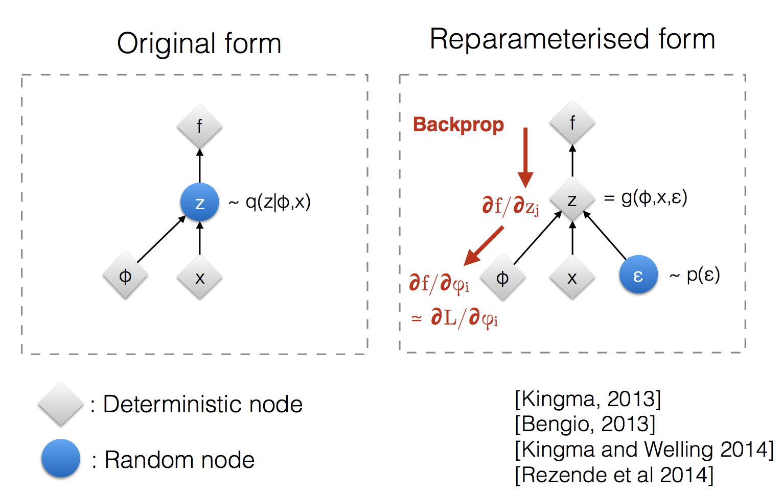
What is the reparameterization trick used in variational autoencoders?
Variational autoencoders sample from \(\mathbf{z} \sim q_\phi(\mathbf{z}\vert\mathbf{x})\).
Sampling is a stochastic process and therefore we cannot backpropagate through it.
To make it differentiable, the reparameterization trick is introduced.
It is often possible to express the random variable \(\mathbf{z}\) as a deterministic variable \(\mathbf{z} = \mathcal{T}_\phi(\mathbf{x}, \boldsymbol{\epsilon})\), where \(\epsilon\) is an auxiliary independent random variable and the transformation function \(\mathcal{T}_\phi\) converts \(\boldsymbol{\epsilon}\) to \(\mathbf{z}\).
For example, a common choice of the form of \(q_\phi(\mathbf{z}\vert\mathbf{x})\) is a multivariate Gaussian with a diagonal covariance structure:
\[\begin{aligned} \mathbf{z} &\sim q_\phi(\mathbf{z}\vert\mathbf{x}^{(i)}) = \mathcal{N}(\mathbf{z}; \boldsymbol{\mu}^{(i)}, \boldsymbol{\sigma}^{2(i)}\boldsymbol{I}) & \\ \mathbf{z} &= \boldsymbol{\mu} + \boldsymbol{\sigma} \odot \boldsymbol{\epsilon} \text{, where } \boldsymbol{\epsilon} \sim \mathcal{N}(0, \boldsymbol{I}) & \scriptstyle{\text{; Reparameterization trick.}} \end{aligned}\]
Draw the architecture of a variational autoencoder (VAE).