Which issues with (mip)-NeRF does mip-NeRF 360 address?
1. (mip)-NeRF struggles with unbounded scenes, mip-NeRF 360 reparameterizes the scenes such that they lay in a bounded space.
2. (mip)-NeRF training requires many iterations and is expensive, mip-NeRF 360 introduces online distillation.
3. (mip)-NeRF has artifacts in large scenes due to ambiguity due to few samples per observation, mip-NeRF 360 adds specific regularization to fix this.
2. (mip)-NeRF training requires many iterations and is expensive, mip-NeRF 360 introduces online distillation.
3. (mip)-NeRF has artifacts in large scenes due to ambiguity due to few samples per observation, mip-NeRF 360 adds specific regularization to fix this.
What is the problem with unbounded scenes in mip-NeRF that mip-NeRF 360 fixes?
mip-NeRF requires bounded rays, as we cannot parameterize an infinite sized ray.
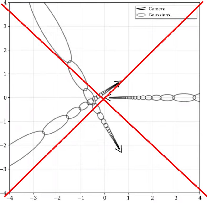
How does mip-NeRF 360 reparameterize the multivariate gaussians that are used to parameterize rays in the original mip-NeRF?
To do this, first let us define \(f(\mathbf{x})\) as some smooth coordinate transformation that maps from \(\mathbb{R}^n \rightarrow \mathbb{R}^n\) (in this case, \(n=3\)). We can compute the linear approximation of this function:
\[f(\mathbf{x}) \approx f(\mathbf{\boldsymbol{\mu}}) + \mathbf{J}_{f}(\mathbf{\boldsymbol{\mu}})(\mathbf{x} - \mathbf{\boldsymbol{\mu}})\]
Where \(\mathbf{J}_{f}(\mathbf{\boldsymbol{\mu}})\) is the Jacobian of \(f\) at \(\boldsymbol{\mu}\). With this, we can apply \(f\) to \((\boldsymbol{\mu}, \boldsymbol{\Sigma})\) as follows:
\[f(\boldsymbol{\mu}, \boldsymbol{\Sigma}) = \left( f(\boldsymbol{\mu}), \, \mathbf{J}_{f}(\mathbf{\boldsymbol{\mu}}) \boldsymbol{\Sigma} \mathbf{J}_{f}(\mathbf{\boldsymbol{\mu}})^\mathrm{T} \right)\]
This is functionally equivalent to the classic Extended Kalman filter, where \(f\) is the state transition model.
Our choice for \(f\) is the following contraction:
\[\operatorname{contract}(\mathbf{x}) = \begin{cases} \mathbf{x} & \|{\mathbf{x}}\| \leq 1\\ \left(2 - \frac{1}{\|{\mathbf{x}}\|}\right)\left(\frac{\mathbf{x}}{\|{\mathbf{x}}\|}\right) & \|{\mathbf{x}}\| > 1 \end{cases}\]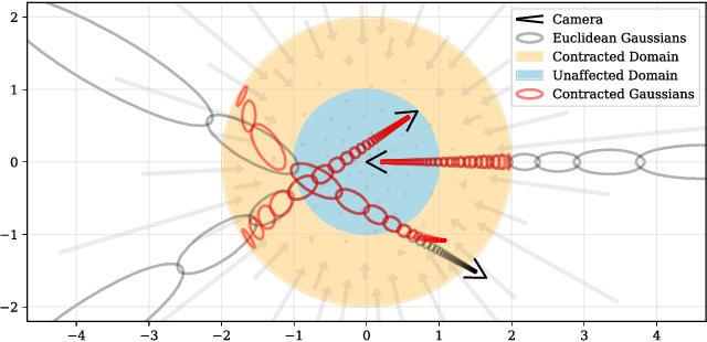
Instead of using mip-NeRF's IPE features in Euclidean space we use similar features in this contracted space: \(\gamma( \operatorname{contract}(\boldsymbol{\mu}, \boldsymbol{Sigma}))\).
How are the rays sampled in mip-NeRF 360?
They are sampled linearly in inverse depth (disparity).
More details in the paper.
Given the following schematic of the mip-NeRF training pipeline,
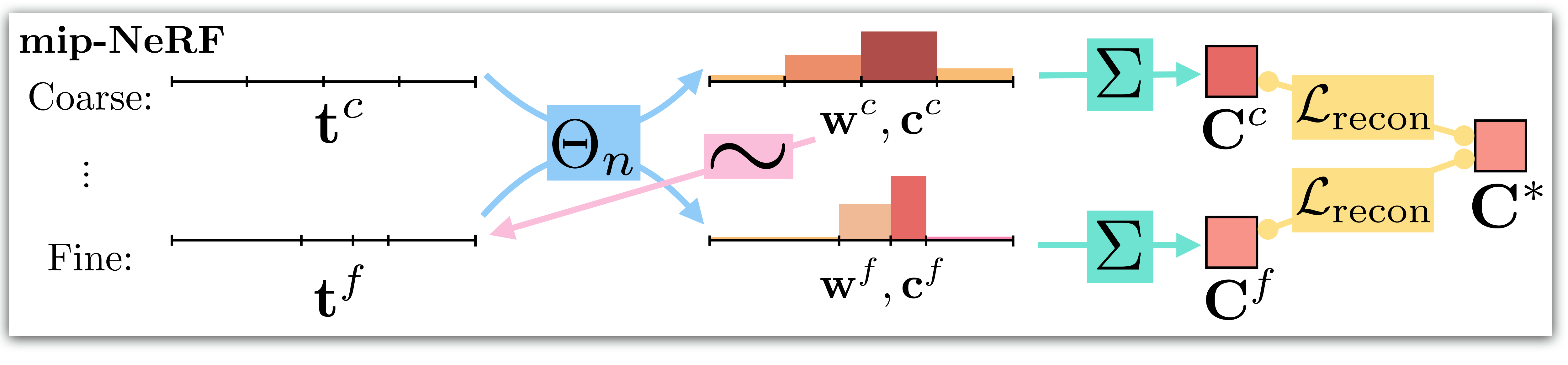
give the schematic of the mip-NeRF 360 pipeline:
give the schematic of the mip-NeRF 360 pipeline:
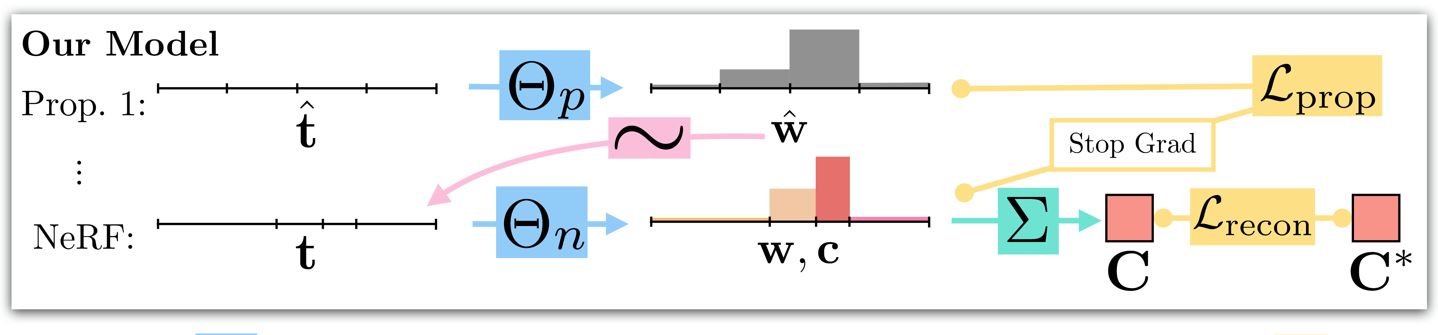
While mip-NeRF uses one multi-scale MLP that is repeatedly queried (only two repetitions shown here) for weights that are resampled into intervals for the next stage, and supervises the renderings produced at all scales. mip-NeRF 360 use a proposal MLP that emits weights (but not color) that are resampled, and in the final stage we use a NeRF MLP to produce weights and colors that result in the rendered image, which we supervise. The proposal MLP is trained to produce proposal weights \(\mathbf{\hat{w}}\) that are consistent with the NeRF MLP’s \(\mathbf{w}\) output. By using a small proposal MLP and a large NeRF MLP we obtain a combined model with a high capacity that is still tractable to train
Which loss function is used to train the proposal MLP used for the online distillation in mip-NeRF 360?
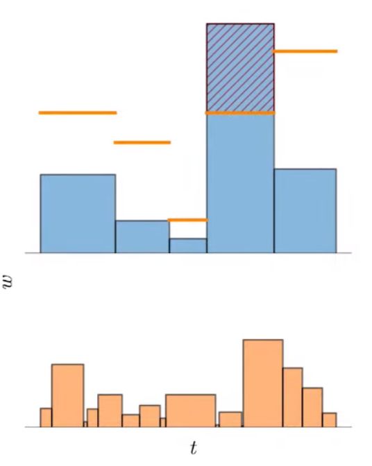
The online distillation requires a loss function that encourages the histograms emitted by the proposal MLP \((\hat{\mathbf{t}}, \hat{\mathbf{w}})\) and the NeRF MLP \((\mathbf{t}, \mathbf{w})\)to be consistent.
If the two histograms are consistent with each other, then it must hold that \(w_i \leq \operatorname{bound}\left( \hat{\mathbf{t}}, \hat{\mathbf{w}}, T_i \right)\) for all intervals \((T_i, w_i)\) in \((\mathbf{t}, \mathbf{w})\) with
\[\operatorname{bound}\left( \hat{\mathbf{t}}, \hat{\mathbf{w}}, T \right) = \sum_{j: \, T \cap \hat{T}_j \neq \varnothing} \hat w_j\]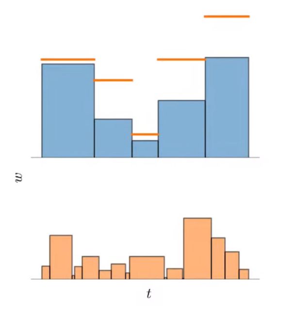
The proposal loss penalizes any surplus histogram mass that violates this inequality and exceeds this bound:
\[\mathcal{L}_{\text{prop}}\left(\mathbf{t}, \mathbf{w}, \hat{\mathbf{t}}, \hat{\mathbf{w}} \right)\!=\! \sum_{i}\frac{1}{w_{i}}\max\left( 0, w_{i} - \operatorname{bound}\left( \hat{\mathbf{t}}, \hat{\mathbf{w}}, T_i \right) \right)^{2}\]
We impose this loss between the NeRF histogram \((\mathbf{t}, \mathbf{w})\) and all proposal histograms \((\hat{\mathbf{t}}^k, \hat{\mathbf{w}}^k)\). A stop-gradient is placed on the NeRF MLP's outputs \(\mathbf{t}\) and \(\mathbf{w}\) when computing \(\mathcal{L}_{\text{prop}}\) so that the NeRF MLP leads and the proposal MLP follows, otherwise the NeRF may be encouraged to produce a worse reconstruction of the scene so as to make the proposal MLP's job less difficult.
What are the artifacts that mip-NeRF 360 tries to avoid with its additional regularization loss?
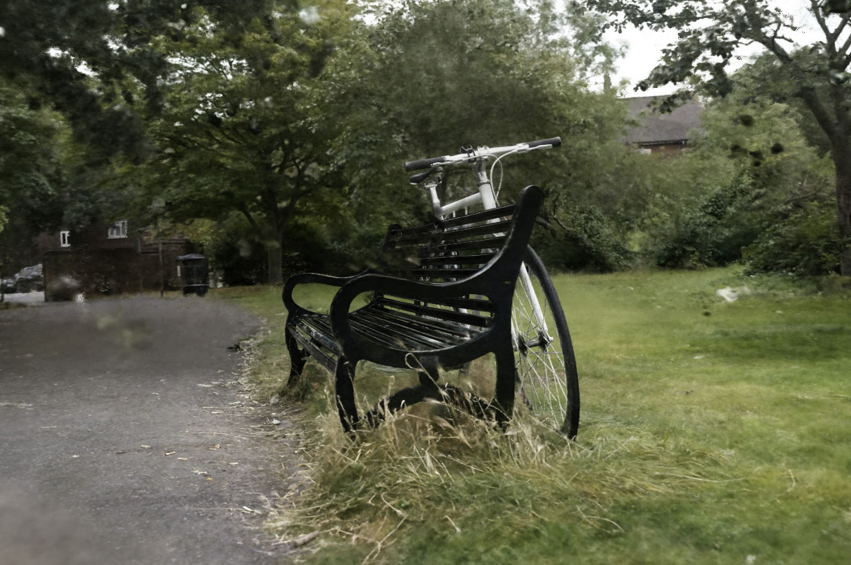
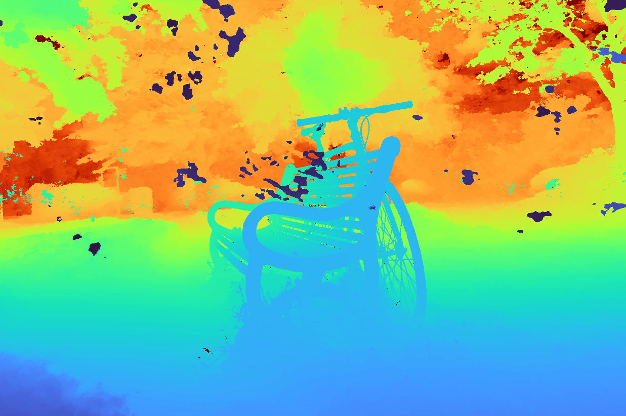
Floaters: the small disconnected regions of volumetrically dense space that look like blurry clouds when viewed from another angle.
Background collapse: is the phenomenon in which distant surfaces are incorrectly modeled as semi-transparent clouds of dense content close to the camera.
Background collapse: is the phenomenon in which distant surfaces are incorrectly modeled as semi-transparent clouds of dense content close to the camera.
How does mip-NeRF 360 eliminate floaters and background collapse artifacts?
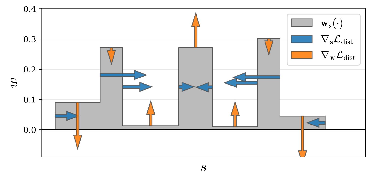
They add a regularizer that is defined in terms of the step function defined by the set of (normalized) ray distances \(\mathbf{s}\) and weights \(\mathbf{w}\) that parameterize each ray:
\[\mathcal{L}_{\text{dist}}(\mathbf{s}, \mathbf{w}) =\iint\limits_{-\infty }^{\,\,\,\infty }\mathbf{w}_\mathbf{s}(u)\mathbf{w}_\mathbf{s}(v) |u - v|\,d_{u}\,d_{v}\]
where \(\mathbf{w}_\mathbf{s}(u)\) is interpolation into the step function defined by \((\mathbf{s}, \mathbf{w})\) at \(u\):
\(\mathbf{w}_\mathbf{s}(u) = \sum_i w_i \mathbb{1}_{[s, s_{i+1})}(u)\).
This loss is the integral of the distances between all pairs of points along this 1D step function, scaled by the weight \(w\) assigned to each point by the NeRF MLP. We refer to this as distortion.
This loss encourages each ray to be as compact as possible by 1) minimizing the width of each interval, 2) pulling distant intervals towards each other, 3) consolidating weight into a single interval or a small number of nearby intervals, and 4) driving all weights towards zero when possible (such as when the entire ray is unoccupied).
Though \(\mathcal{L}_{\text{dist}}\) is straightforward to define, it is non-trivial to compute.
But because \(\mathbf{w}_\mathbf{s}(\cdot)\) has a constant value within each interval we can rewrite it as:
\[\begin{align} \mathcal{L}_{\text{dist}}(\mathbf{s}, \mathbf{w}) &= \sum_{i,j} w_{i} w_{j} \left| \frac{s_{i} +s_{i+1}}{2} - \frac{s_{j} + s_{j+1}}{2} \right| \nonumber \\ &+ \frac{1}{3}\sum _{i} w_{i}^{2}( s_{i+1} - s_{i}) \end{align}\]