What problem with NeRFs does Mip-NeRF solve?
The original NeRF's rendering procedure can lead to aliasing artifacts when rendering content from multiple resolutions (e.g. zoomed in or out).
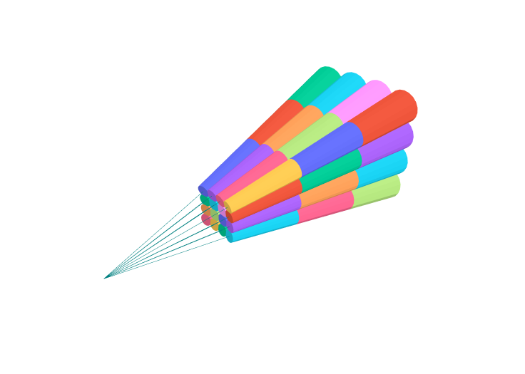
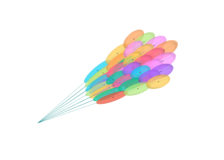
Example: Nerf (left) vs Mip-NeRF (right):
How does Mip-NeRF extend NeRF's representation?
Mip-NeRF extends NeRF to represent the scene at a continuously-valued scale, By efficiently rendering anti-aliased conical frustums instead of rays.


In Mip-NeRF how are the conical frustrums modelled such that they can be efficiently used in NeRFs?
The conical frustrums are approximated with multivariate Gaussians.


These gaussians are fully characterized by the mean distance along the ray \(\mu_t\), the variance along the ray \(\sigma^2_t\) and the variance perpendicular to the ray \(\sigma^2_r\).
\[\mu_t = t_\mu + \frac{2 t_\mu t_\delta^2}{3 t_\mu^2 + t_\delta^2}\]
\[\sigma_t^2 = \frac{t_\delta^2}{3} -\frac{4 t_\delta^4 (12 t_\mu^2 - t_\delta^2)}{15 (3 t_\mu^2 + t_\delta^2)^2}\]
\[\sigma_{r}^2 = r^2 \left( \frac{t_\mu^2}{4} + \frac{5 t_\delta^2}{12} - \frac{4 t_\delta^4}{15 (3 t_\mu^2 + t_\delta^2)} \right)\]with \(t_\mu = (t_{\text{start}} + t_{\text{end}})/2\) and \(t_\delta = (t_{\text{end}} + t_{\text{start}})/2\) and the radius \(r\) the width of the pixel in world coordinates scaled by \(2/\sqrt{12}\).
Applying this to a ray gives the final guassian characteristics:
\[\mathbf{\mu} = \mathbf{o} + \mu_t\mathbf{d}, \Sigma = \sigma^2_t(\mathbf{dd}^\top) + \sigma^2_r \left( \mathbf{I} - \frac{\mathbf{dd}^top}{||\mathbf{d}||^2_2} \right)\]
See paper appendix for full derivation of the above formulas.
How are the multivariate Gaussians in Mip-NeRF converted to inputs for the NeRF?
The multivariate Gaussians are transformed to integrated positional encodings (IPE).
This is the expected value of the positional encodings of samples from mulitvariate Gaussian.
\[\begin{align} \gamma(\boldsymbol{\mu}, \Sigma) &= \mathbb{E}_{\mathbf{x} \sim \mathcal N(\boldsymbol{\mu}_\gamma, \Sigma\gamma)}\left[\gamma(\mathbf{x})\right] \\ &= \begin{bmatrix} \sin(\boldsymbol{\mu}_\gamma) \circ \exp\left(-(\frac{1}{2}) \operatorname{diag}\left(\Sigma_\gamma\right)\right) \\ \cos(\boldsymbol{\mu}_\gamma) \circ \exp\left(-(\frac{1}{2}) \operatorname{diag}\left(\Sigma_\gamma\right)\right)\end{bmatrix} \end{align}\]